DEPARTMENT OF ELECTRONIC & ELECTRICAL ENGINEERING
LIQUID CRYSTAL MODELLING

INFORMATION FOR

Prospective Students
Current Students

INFORMATION

Home
Group Members
Modelling
Devices
Downloads
Publications

PROJECTS

Funded
Undergraduate
Postgraduate

QUICK LINKS

Optical Devices
Ghent LC Group
GID

Liquid Crystal Hydrodynamics with Variable Order

When disclinations are present, the LC ordering becomes biaxial near the core and the order parameter drops (as represented by the background colour of the figure to the right). We have developed Finite Element discretisations of the Qian-Sheng Equations in both 2D and 3D. The Qian-Sheng equations are a generalisation of Ericksen-Leslie theory for LC hydrodynamics to include changes in the order parameter [1]. The Finite Element Method is well suited to resolve the rapid variations in order parameter about disclination whilst still being able to model large container sizes.

Three elastic constants
Flexo-electric effect
Anisotropic weak anchoring [2]

Theory

The order and the orientation of the liquid crystal are represented by a symmetric and traceless tensor, the Q-tensor:

$\mathbf{Q}:=S_1 \left(3\hat{n}\otimes\hat{n}-I\right)/2+S_2 \left(3\hat{m}\otimes\hat{m} -I\right)/2,$

where and represent the degree of order about the vectors $\hat{n}$ and $\hat{m}$ respectively.

The equilibrium Q-tensor field minimizes the Landau-de Gennes (LdG) free energy functional:

${\cal F}(\mathbf{Q}) := \int_\Omega \{ f_D(\partial \mathbf{Q})+f_B(\mathbf{Q})-f_E(\mathbf{Q}) \} + \int_\Gamma \{ f_S (\mathbf{Q})\},$

where $\Omega$ is an open bounded subset of $\mathbb{R}^3$ with boundary $\Gamma$ . The free-energy densities $f_D(\partial\mathbf{Q})$ and $f_E(\mathbf{Q})$ are due to elastic and electrostatic contributions respectively and $f_S(\mathbf{Q})$ is the surface free-energy density. The bulk free-energy density $f_B(\mathbf{Q})$ constrains the degree of order of the LC:

$f_B(\mathbf{Q}):=\frac{1}{2}A {\rm tr}(\mathbf{Q}^2) + \frac{1}{3}B{\rm tr}(\mathbf{Q}^3) + \frac{1}{4}C{\rm tr}(\mathbf{Q}^2)^2$

$f_D(\partial \mathbf{Q}):=\frac{1}{2}L_1 Q_{\alpha\beta,\gamma} Q_{\alpha\beta,\gamma} + \frac{1}{2}L_2 Q_{\alpha\beta,\beta} Q_{\alpha\gamma,\gamma} \\ +\frac{1}{2}L_4\sigma_{\alpha\beta\lambda}Q_{\alpha\gamma}Q_{\beta \gamma,\lambda}+\frac{1}{2}L_6 Q_{\alpha\beta}Q_{\gamma\lambda,\alpha}Q_{\gamma\lambda,\beta}$

$f_E(\mathbf{Q}) := \frac{1}{2} \varepsilon_0 (\nabla u \cdot \bar{\bar{\varepsilon}} \cdot \nabla u)-\vec{P}\cdot\nabla u$

where , and are thermotropic constants, to are elastic constants, $\sigma_{\alpha\beta\lambda}$ is the Levi-Civita anti-symmetric tensor and is the electric potential. Here, the saddle-splay modulus has been neglected. The flexoelectric polarization $\vec{P}$ can be defined as

$\vec{P}(\partial\mathbf{Q}) := \epsilon_1 (\nabla\cdot\mathbf{Q}) + \epsilon_2 \mathbf{Q}\cdot(\nabla\cdot\mathbf{Q}).$

The surface contribution takes the form [2]

$f_S(\mathbf{Q}):=a{\rm tr}(\mathbf{Q}^2) + W_1 (\hat{\xi_1}\cdot\mathbf{Q}\cdot\hat{\xi_1}) + W_2 (\hat{\xi_2}\cdot\mathbf{Q}\cdot\hat{\xi_2}).$

This is an anisotropic anchoring energy; a different energy penalty can be assigned to azimuthal and zenithal perturbations from the preferred (easy) alignment direction. The first term is necessary to maintain the surface order parameter, $\xi_1$ and $\xi_2$ are unit vectors orthogonal to the easy direction and and are anchoring strengths. A more complete description of the anchoring types supported by this expression and a means to calculate the coefficient can be found in [2].

Implementation [3]

The implementation is well suited to the modelling of defect movement in realistically sized geometries, via the following features:

Adaptive meshing scheme based on an empirical error estimate
Crank-Nicholson time integration using a variable time step
Matrices calculated using Gauss integration, allowing curved edge elements to be used

This implicit scheme leads to a larger memory use than the constant order program. However, the rapid spatial variations in the order parameter near disclinations severely limits the time step for explicit methods (<1ns!). We prefer the implicit method in this case to achieve reasonable simulation times. Flow of the liquid crystal is calculated by solving the Navier-Stokes equations with a stress tensor that takes into account the anisotropy of the LC.

The following assumptions are made:

Liquid crystal is incompressible
Low-Reynold's number approximation
Electric potential and velocity fields are pseudo-steady with respect to the changing Q-tensor

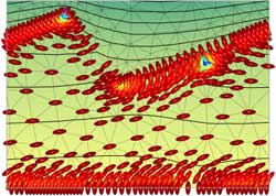
These assumptions could be dropped if required, at the cost of an increase in simultion time.

The 2D and 3D implementations differ. In 2D second order shape functions are used for the Q-tensor, velocity and electric potential. A mixed interpolation is used for the Navier-Stokes equation to avoid oscillatory pressure solutions. Therefore first order shape functions are used for the pressure. In 3D first order shape functions are used for all variables, and a stabilized form of the Navier-Stokes equations.

Results

Fig. 1 shows an example simultion results for a type of bistable display device.

Fig. 1: Defect movement in a Zenithally Bistable Nematic (ZBN) style device, with a negative dielectric anisotropy liquid crystal (director colour represents the order parameter)

[1] T. Qian and P. Sheng, “Generalized hydrodynamic equations for nematic liquid
crystals,” Physical Review E, vol. 58, no. 6, pp. 7475–7485, 1998.

[2] E. Willman, F. A. Fern´andez, R. James, and S. E. Day, “Phenomenological
anisotropic anchoring energy of nematic liquid crystals for the Landau-de Gennes
theory,” to appear in IEEE Transactions on Electron Devices.

[3] R. James, E. Willman, F. A. Fernandez, and S. E. Day, “Finite-element modeling
of liquid-crystal hydrodynamics with a variable degree of order,” IEEE Transactions
on Electron Devices, vol. 53, no. 7, pp. 1575–1582, 2006.

This page last modified 8 July, 2007 by r.james