DEPARTMENT OF ELECTRONIC & ELECTRICAL ENGINEERING
LIQUID CRYSTAL MODELLING

INFORMATION FOR

Prospective Students
Current Students

INFORMATION

Home
Group Members
Modelling
Devices
Downloads
Publications

PROJECTS

Funded
Undergraduate
Postgraduate

QUICK LINKS

Optical Devices
Ghent LC Group
GID

1D Matlab Liquid Crystal Solver

This page describes a simple Matlab based 1D solver to find the steady state liquid crystal orientation, using the Matlab Boundary Value Problem (BVP) solver, bvp4c. The theory and implementation is described using a one elastic constant formulation. A full three elastic constant formulation is available for download.

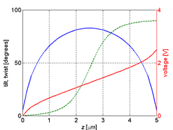
Fig. 1: Tilt, twist and voltage distributions in a twisted nematic (TN) cell

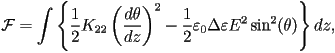
One Elastic Constant Formulation

The Oseen-Frank free energy may be written as

${\cal F} = \int\left\{ \frac{1}{2}K_{22}\left(\frac{d\theta}{dz}\right)^2-\frac{1}{2}\varepsilon_0 \Delta\varepsilon E^2 \sin^2(\theta)\right\}dz,$

assuming there is no twist of the liquid crystal, where $K_{22}$ is the elastic constant, $\Delta\varepsilon$ is the dielectric anisotropy, $\theta(z)$ is the tilt and is the electric field. The equilibrium value of the function $\theta(z)$ is such that it minimizes the functional ${\cal F}.$

Taking first order variations we find that $\theta(z)$ must satisfy the following differential equation

$K_{22} \frac{d^2\theta}{dz^2}+\varepsilon_0 \Delta\varepsilon E^2 \sin(\theta)\cos(\theta) = 0.$

This is a second order differential equation. To solve this using the Matlab BVP solver, it must first be converted into two first order equations by introducing an extra variable. Following the approach shown here; setting $\theta(z)\rightarrow\theta_1$ and $\theta'(z)\rightarrow\theta_2$ gives a set of two coupled linear differential equations :

$\theta'_1=\theta_2$

$K_{22} \theta'_2+\varepsilon_0 \Delta\varepsilon E^2 \sin(\theta_1)\cos(\theta_1) = 0.$

Things aren't quite that simple though. As the liquid crystal reorients the permittivity changes, which affects the electric field. In fact the electric field should be calculated too, by solving the Laplace equation:

$\nabla \cdot \overline{\overline{\varepsilon}} \cdot \nabla u = 0,$

where

is the potential and $E=-\nabla u$ . Since we only have a 1D problem this reduces to

$\frac{d}{dz}\left[\varepsilon_{zz} \frac{du}{dz}\right] = 0,$

with $\varepsilon_{zz}=\varepsilon_\perp + \Delta\varepsilon \sin^2\theta$ . Applying the chain differentiation rule gives

$2\Delta\varepsilon \sin(\theta)\cos(\theta)\frac{d\theta}{dz}\frac{du}{dz}+[\varepsilon_\perp + \Delta\varepsilon \sin^2(\theta)]\frac{d^2u}{dz^2}=0.$

Once again this is a second order equation which must be linearised by introducing $u(z)\rightarrow u_1$ and $u'(z)\rightarrow u_2$ gives

$\theta'_1=\theta_2$

$K_{22} \theta'_2+\varepsilon_0 \Delta\varepsilon u_2^2 \sin(\theta_1)\cos(\theta_1) = 0$

$2\Delta\varepsilon \sin(\theta_1)\cos(\theta_1)\theta_2 u_2+[\varepsilon_\perp + \Delta\varepsilon \sin^2(\theta_1)]u'_2=0.$

This set of four linear differential equations can be solved for in terms of the vector

$\{\theta'_1,\theta'_2,u'_1,u'_2\}.$

Three Elastic Constant Formulation

With three elastic constants the free energy functional is supplemented by terms that account for the splay-bend anisotropy of the liquid crystal There are three elastic constants $K_{11}$ , $K_{22}$ and $K_{33}$ , which correspond to splay, twist and bend deformations:

${\cal F} = \int_\Omega\left\{\frac{1}{2} K_{11}(\nabla\cdot\hat{n})^2+\frac{1}{2}K_{22}(\hat{n}\cdot\nabla\times\hat{n})^2 +\frac{1}{2}K_{33}|\hat{n}\times\nabla\times\hat{n}|^2-\frac{1}{2}\varepsilon_{0}(\vec{E}\cdot\overline{\overline{\varepsilon}}\cdot\vec{E})\right\}$

The derivation, following the steps outlined in the previous section, is rather tedious. Instead one may use Maple to generate the equations.

The Maple code can be downloaded here: lc3k.mws. I'm still learning Maple, so this code could be improved.

This program solves for both the tilt and twist, $\phi(z)$ , of the liquid crystal, using the vector:

$\{\theta'_1,\theta'_2,\phi'_1,\phi'_2,u'_1,u'_2\}.$

The function may be called as follows

[z,theta,phi,u] = lc3k(volts);

where z is a vector containing the locations of the mesh points, theta is the tilt, phi is the twist and u is the potential. It is assumed that a potential difference of volts is applied across the cell. Currently the material constants are hard coded into the function lc3k. Modify the program to take these as arguments if you wish.

Currently the initial condition for the tilt is set to quadratic to improve convergence:

$\theta\propto z(1-z), \mbox{~where~} z \mbox{~lies in~}[0,1].$

In this latest version, alignment layers of finite thickness are supported. The left and right alignment layers may be of different thicknesses and relative permittivities. The thickness may also be set to zero.

Anchoring may be strong or weak at the left and right alignment layers. Set W = Inf for strong anchoring. The anchoring energy is assumed isotropic and takes the form Fs = -W/2*(n.n0)^2.

Warning: Since the implementation uses polar angles, it does not work well for large voltages as the twist becomes degenerate, leading to a singular Jacobian matrix. One way to avoid this problem is to discretise the equations in terms of the components of the director. A problem with this approach is that the unitary length of the director must in some way be enforced. This tends to increase the order of the governing equations and has a detrimental effect on the convergence.

A simple Jones code calulates the optical transmittance.

Finally, the Matlab code can be found here: lc3k.m.

Dynamic Formulation

Additionally, a dynamic formulation, where the rate of change of the free energy is mediated by the rotational viscosity, gamma1, is available below. The solution is sought using the Matlab initial-boundary value solver for parabolic-elliptic PDEs, PDEPE. Weak anchoring and alignments layers are supported.

This formulation is somewhat slower that the steady-state solver above. However, it is more stable, since it does not require the initial condition to be close to the desired solution.

The Matlab code can be found here: lc3kdt.m.

This page last modified 16 April, 2010 by r.james