LCview - Liquid Crystal 2D/3D Visualisation

This program visualises results on both irregular and regular 2D and 3D meshes and is the product of many years development here at UCL. Written in C++ using MFC and OpenGL and is available for Windows only.

Director field can be plotted over cut planes
Iso-surface plots: Voltage, Order Parameter, Twist, Tilt, etc.
Image, contour and surface plots
Built in extended Jones optics code
Viewing angle plots
Fast conversion from irregular to regular meshes
Export AVI movies
Free energy calculation

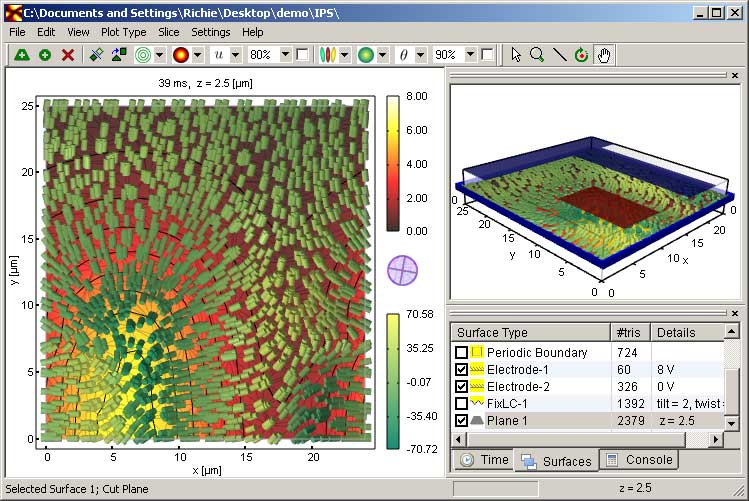
A guide to using the program can be found here. Fig. 1 shows a screen shot of the program. The left hand view displays the director and potential field on a cut plane. The top right hand view is a sketch of the 3D structure with a the cut plane displayed, which can be repositioned using the mouse. The bottom right hand view is a list of result files in the current directory. Typically each file corresponds to a simulation result at a particular time. This view allows the user to quickly change the result file/time the is being viewed.

Fig.1: Screenshot of LCview program (click to enlarge)

Although the program is designed to visualise director fields at snapshots in time, it has the facility to calculate the transmittance as a function of time (see this page for more information). It is possible to convert all the results in a given director from irregular to regular meshes. These results can then be easily parsed in Matlab to produce plots of Voltage, Tilt and Twist against time (see this page for more information). Future versions of the program should extend these facilities.

3D simulations are usually performed using meshes which contain many nodes. Plotting the director at each node would result in a mess of overlapping cylinders. Usually we are concerned only with the director field over one or more cut planes or surfaces. The 3D Mesh View provides a means to add, move and rotate cut planes using the mouse.

Fig.2: Selecting and moving a cut plane

Fig. 2 shows a cut plane being selected, moved and then rotated. For every cut the user can choose the:

scalar parameter represented by the cut plane colour: Voltage, Order Parameter, Twist, Tilt, etc.
whether or not to plot director or flow fields
scalar parameter represented by the director colour: Order Parameter, Twist, Tilt, etc.
cut plane and director colour map
transparency of the cut plane and director

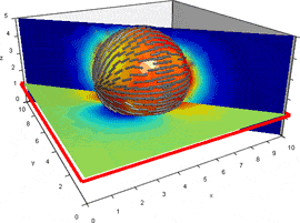
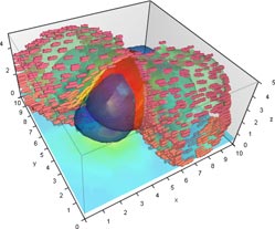
These choices are made using the 'Slice/Cut Properties' Toolbar. The surface meshes produced by the mesh generator can be selected just like any cut plane can. The user can then choose from the properties of the surface from the list above. The sphere is Fig.2 is present in the GID mesh and represents a cylindrical spacer with planar degenerate anchoring over the surface. Here, the surface has been selected, directors enabled, and the colour changed to represent the tilt.

Fig.3: Director field about a spherical spacer

The user can manipulate the view using:

Rotate view: Hold left mouse button and move mouse
Select a cut plane or mesh surface: Left click
Move a selected cut plane: Right mouse button
Change selected cut plane normal: Double left click or from menu Edit-Edit Slice Normal

The links below describe in more detail how to use the program.

Getting Started
Plot types
Converting from an irregular to a regular mesh
Calculating the optical transmittance
Calculating the free energy

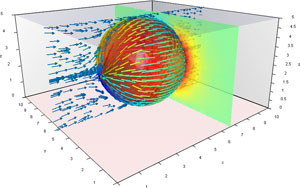
Fig. 3 and 4 show some examples of different visualisation's of the same structure and more examples follow.

Fig.4: Director field about a spherical spacer (with off-axis cuts)

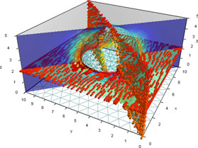
Fig.5: Iso-surfaces about a spherical spacer. Iso-Surfaces properties can be modified in the same way as cut planes

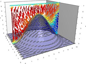
Fig.6: Director field about a microlens

Fig.7: A +1/2 disclination line. Directors are plotted as cylinders in the uniaxial state, but when the LC is biaxial, the LC orientation is represented by cuboids

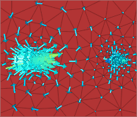
Fig.8: Flow field due to pair annihilating disclination lines of strength 1/2

Fig.9: Flow field represented by injected particles

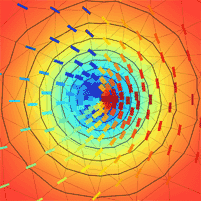
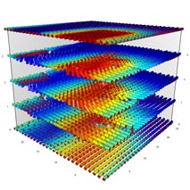
Fig.10: Equi-potential surfaces and director field in a Spatial Light Modulator

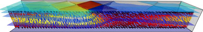
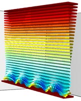
Fig.11: Director stack plot and equi-potential surfaces in an IPS cell

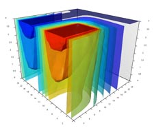
Fig.12: Director field in a device where fringing fields between electrodes reorient the LC

This page last modified 6 October, 2006 by r.james