|

| INFORMATION FOR Prospective Students INFORMATION Home PROJECTS Funded QUICK LINKS Optical Devices
|
Three Dimensional Director Modelling
 The computer modelling group at UCL has many years experience
in Electromagnetics, and Liquid Crystal Modelling. As a product of
this work a program has been developed, which is applicable to a wide
range of LC geometries. A CAD program is used to produce the mesh,
supporting complex shaped volumes, and curved alignment surfaces and
electrodes. The computer modelling group at UCL has many years experience
in Electromagnetics, and Liquid Crystal Modelling. As a product of
this work a program has been developed, which is applicable to a wide
range of LC geometries. A CAD program is used to produce the mesh,
supporting complex shaped volumes, and curved alignment surfaces and
electrodes.A variational approach to the Oseen-Frank free energy is taken, discretised using finite elements on a mesh of tetrahedral elements. A variable time step is used to accelerate the computation.
A simple interface provides a means to configure the material properties, and gives a graphical indication of the progress of the simulation. Ion transport within the the LC can be taken into account in this model, by algorithms produced at the University of Gent. In addition a constant charge formulations is available, as well as two-dimensional finite element and finite difference implementations. If you are interested in obtaining any of the programs detailed here, please feel free to email me. If you have any problems using the program please check the troubleshooting page which details some common mistakes. Defining the Cell Geometry WinLCD runs on a mesh of tetrahedral elements. A choice
of two mesh generator is available GID and Tetgen. WinLCD runs on a mesh of tetrahedral elements. A choice
of two mesh generator is available GID and Tetgen.
GID has a CAD like interface which allows complex structure to be drawn. An academic version can be downloaded and used for free, but there is a limit on the number of elements it can generate, and so it is only feasible to model simple structures. The professional version removes this limit, and is reasonably priced. http://gid.cimne.upc.es/download/ An alternative is to use TetGen which uses input files as opposed to a GUI which makes inputting of complex structures more difficult, although it can take surface meshes from programs such as GID. It produces high quality meshes and the author, Hang Si, is responsive to questions and is very helpful. Tetgen is free, but has its own licence restrictions which can be viewed on the TetGen website. There is no limit on the number of elements it can produce. The documentation and source code for TetGen can be found at the
following location:
Creating a Planar Cell and Meshing
Before the physical structure is defined it is usual to introduce the types of volumes supported the program as well as the boundary conditions that can be applied to surfaces. A material number is assigned to all surfaces and volumes that we define. There are two supported types of volumes dielectric and LC volumes. A structure may contain up to 7 different types of dielectric and 7 types of LC material! There are more types of surfaces that can be defined. An LC device will have alignment layers which are treated in some way, giving a preferred direction of orientation at the surface. A surface may be specified as an alignment surface by applying a material number FixLC-x, where x={1,2,..}. There will be some energy penalty associated with deflection from this preferred direction, the magnitude of which depends on the surface treatment. The nature of the alignment on the surface is specified in elastic.i, which will be discussed in more detail in the next section. Devices will also contain electrodes to reorient the LC. Any surface can be assigned as an electrode using the material names Electrode-x. In a real device the alignment layer is a thin insulating layer that separates the LC from the electrodes or glass substrate. If the alignment layer is sufficiently thin compared to the thickness of the LC layer it is possible to fix the LC director and pin the potential on the same surface mesh. To describe such surfaces will dual behaviour it is necessary to be able to combine material name, e.g. FixLC-1_Electrode-2. This method is necessary because two material numbers can't be applied to a surface. In GID the user only needs to know the material names discussed above. So that GID knows these names, a problem_type is required, which can be downloaded here. This zip file contains a directory that should be copied into the GID problem type directory. In Tetgen the user is required to know the actual material number, which can be derived from the material number using the table below, which specifies the bits of the number that represent each property. For example if bit 128 only of the material number is set, the corresponding name is Electrode-2
There structure must fulfull one requirement. The program expects the LC layer to extend in x-y plane. This assumption is in face only used when setting the initial director configuration and will probably be removed in a future revision. For a simple structure this means that aliment surfaces will be normal to z. The following form can be used to find the material numbers (requires JavaScript):
For more GID tips click here. For more advanced structures click here
To create a simple structure with Tetgen click here To create a more complex IPS stucture in Tetgen click here
After following these instruction the mesh will have been generated. A text file mesh.txt will be obtained containing a list of node, tetrahedra and triangles.
Input Files: Material Properties and Voltage Waveforms
Running the Simulation A simulation directory must contain 4 files
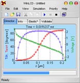
The first three files should be configured as described above, then load up WinLCD, press Play and wait! As the program runs it will output result files at the result look times specfied in voltdata.i. The file names will be of the form resultxxx.dat. These files contain the director and potential values at each node of the mesh. The program will run until the last look time is reached or until the user closes the program. If the program is accidenttally closed, a simulation can be restarted from an existing result file. Just modify the 6th line of voltdata.i. Viewing Results The result files can be opened up in Matlab using the code available here, or the Visualisation Program, which can be found here.
[1] W. Zhao, C.-X. Wu, and M. Iwamoto, “Analysis of weak-anchoring effect in nematic liquid crystals,” Phys. Rev. E, vol. 62, no. 2, pp. 1481–1484, 2000. This page last modified 10 November, 2006 by r.james |
|||||||||||||||||||||||||||||||||||
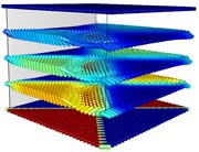
 The solution for the
director is alternated within each time step with the calculation
of the potential, and is iterated until a consistent solution is
achieved.
The solution for the
director is alternated within each time step with the calculation
of the potential, and is iterated until a consistent solution is
achieved. Complex 3D geometries can be modelled, but to demonstrate
how to use the programs we begin with a simple planar structure.
Complex 3D geometries can be modelled, but to demonstrate
how to use the programs we begin with a simple planar structure.