|
Constructors
|
|
public Regression(double[ ][ ] xdata, double[ ] ydata, double[ ] yErrors)
|
public Regression(double[ ][ ] xdata, double[ ] ydata, double[ ][] xerrors, double[ ] yerrors)
|
public Regression(double[ ][ ] xdata, double[ ][] ydata, double[ ][ ] yerrors)
|
public Regression(double[ ][ ] xdata, double[ ][] ydata, double[ ][ ] xerrors, double[ ][ ] yerrors)
|
|
public Regression(double[ ] xdata, double[ ] ydata, double[ ] yErrors)
|
|
public Regression(double[ ] xdata, double[ ] ydata, double[ ] xerrors, double[ ] yerrors)
|
|
public Regression(double[ ] xdata, double[ ][] ydata, double[ ][ ] yerrors)
|
|
public Regression(double[ ] xdata, double[ ][] ydata, double[ ] xerrors, double[ ][ ] yerrors)
|
|
public Regression(double[ ][ ] xdata, double[ ] ydata)
|
|
public Regression(double[ ][ ] xdata, double[ ][] ydata)
|
|
public Regression(double[ ] xdata, double[ ] ydata)
|
|
public Regression(double[ ] xdata, double[ ][] ydata)
|
|
public Regression(double[ ] xdata, double binWidth, double binZero)
|
|
public Regression(double[ ] xdata, double binWidth)
|
Linear
Regression
|
Fitting to a constant
yi = a0
|
public void constant()
|
public void constantPlot()
public void constantPlot(String xLegend, String yLegend)
|
Linear with intercept
yi = a0+a1.x0,i+a2.x1,i+...
|
public void linear()
public void linear(double fixedIntercept)
|
public void linearPlot()
public void linearPlot(double fixedIntercept)
public void linearPlot(String xLegend, String yLegend)
public void linearPlot(double fixedIntercept, String xLegend, String yLegend)
|
General linear
yi = a0.f1(x0,x1..)+a1.f2(x0,x1+...)
|
public void linearGeneral()
|
public void linearGeneralPlot()
public void linearGeneralPlot(String xLegend, String yLegend)
|
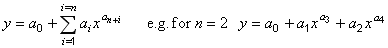
Polynomial
yi = a0+a1.x+a2.x2+a3x3 ...
|
public void polynomial(int n)
public void polynomial(int n, double fixedIntercept)
|
public void polynomialPlot(int n)
public void polynomialPlot(int n, double fixedIntercept)
public void polynomialPlot(int n, String xLegend, String yLegend)
public void polynomialPlot(int n, double fixedIntercept, String xLegend, String yLegend)
|
public ArrayList<Object> bestPolynomial()
public ArrayList<Object> bestPolynomial(double fixedIntercept)
|
public ArrayList<Object> bestPolynomialPlot()
public ArrayList<Object> bestPolynomialPlot(double fixedIntercept)
public ArrayList<Object> bestPolynomialPlot(String xLegend, String yLegend)
public ArrayList<Object> bestPolynomialPlot(double fixedIntercept, String xLegend, String yLegend)
|
public void setFtestSignificance(double signif)
public double getFtestSignificance()
|
public void nonIntegerPolynomial(int nTerms) [non-linear regression]
|
public void nonIntegerPolynomialPlot(int nTerms) [non-linear regression]
public void nonIntegerPolynomialPlot(int nTerms, String xLegend, String yLegend)
|
|
Return the best estimates
|
public double[] getBestEstimates()
|
|
Return the errors of the best estimates
|
public double[] getBestEstimatesErrors()
|
|
See Common methods for list of methods associated with performing a linear regression, e.g. returning a statistical analysis of a linear regression, plotting the best fit curve.
|
Non-linear
Regression
WARNING
|
Nelder and Mead Simplex
One set of dependent variables
y = f(a0,a1,a2..., x0,x1,x2...)
Several sets of the dependent variable
y0 = f1(a0,a1,a2..., x0,x1,x2...)
y1 = f2(a0,a1,a2..., x0,x1,x2...)
. . .
yn = fn(a0,a1,a2..., x0,x1,x2...)
|
public void simplex(RegressionFunction rf, double[ ] start, double[ ] step, double ftol, int nmax)
public void simplex(RegressionFunction rf, RegressionDerivativeFunction rdf, double[ ] start, double[ ] step, double ftol, int nmax)
public void simplex(RegressionFunction2 rf, double[ ] start, double[ ] step, double ftol, int nmax)
public void simplex(RegressionFunction2 rf, RegressionDerivativeFunction2 rdf, double[ ] start, double[ ] step, double ftol, int nmax)
public void simplex(RegressionFunction3 rf, double[ ] start, double[ ] step, double ftol, int nmax)
public void simplex(RegressionFunction3 rf, RegressionDerivativeFunction rdf, double[ ] start, double[ ] step, double ftol, int nmax)
public void simplex(RegressionFunction3 rf, RegressionDerivativeFunction2 rdf, double[ ] start, double[ ] step, double ftol, int nmax)
|
public void simplexPlot(RegressionFunction rf, double[ ] start, double[ ] step, double ftol, int nmax)
public void simplexPlot(RegressionFunction rf, RegressionDerivativeFunction rdf, double[ ] start, double[ ] step, double ftol, int nmax)
public void simplexPlot(RegressionFunction2 rf, double[ ] start, double[ ] step, double ftol, int nmax)
public void simplexPlot(RegressionFunction2 rf, RegressionDerivativeFunction2 rdf, double[ ] start, double[ ] step, double ftol, int nmax)
public void simplexPlot(RegressionFunction3 rf, double[ ] start, double[ ] step, double ftol, int nmax)
public void simplexPlot(RegressionFunction3 rf, RegressionDerivativeFunction rdf, double[ ] start, double[ ] step, double ftol, int nmax)
public void simplexPlot(RegressionFunction3 rf, RegressionDerivativeFunction2 rdf, double[ ] start, double[ ] step, double ftol, int nmax)
|
public void simplex(RegressionFunction rf, double[ ] start, double[ ] step, double ftol)
public void simplex(RegressionFunction rf, RegressionDerivativeFunction rdf, double[ ] start, double[ ] step, double ftol)
public void simplex(RegressionFunction2 rf, double[ ] start, double[ ] step, double ftol)
public void simplex(RegressionFunction2 rf, RegressionDerivativeFunction2 rdf, double[ ] start, double[ ] step, double ftol)
public void simplex(RegressionFunction3 rf, double[ ] start, double[ ] step, double ftol)
public void simplex(RegressionFunction3 rf, RegressionDerivativeFunction rdf, double[ ] start, double[ ] step, double ftol)
public void simplex(RegressionFunction3 rf, RegressionDerivativeFunction2 rdf, double[ ] start, double[ ] step, double ftol)
|
public void simplexPlot(RegressionFunction rf, double[ ] start, double[ ] step, double ftol)
public void simplexPlot(RegressionFunction rf, RegressionDerivativeFunction rdf, double[ ] start, double[ ] step, double ftol)
public void simplexPlot(RegressionFunction2 rf, double[ ] start, double[ ] step, double ftol)
public void simplexPlot(RegressionFunction2 rf, RegressionDerivativeFunction2 rdf, double[ ] start, double[ ] step, double ftol)
public void simplexPlot(RegressionFunction3 rf, double[ ] start, double[ ] step, double ftol)
public void simplexPlot(RegressionFunction3 rf, RegressionDerivativeFunction rdf, double[ ] start, double[ ] step, double ftol)
public void simplexPlot(RegressionFunction3 rf, RegressionDerivativeFunction2 rdf, double[ ] start, double[ ] step, double ftol)
|
public void simplex(RegressionFunction rf, double[ ] start, double[ ] step, int nmax)
public void simplex(RegressionFunction rf, RegressionDerivativeFunction rdf, double[ ] start, double[ ] step, int nmax)
public void simplex(RegressionFunction2 rf, double[ ] start, double[ ] step, int nmax)
public void simplex(RegressionFunction2 rf, RegressionDerivativeFunction2 rdf, double[ ] start, double[ ] step, int nmax)
public void simplex(RegressionFunction3 rf, double[ ] start, double[ ] step, int nmax)
public void simplex(RegressionFunction3 rf, RegressionDerivativeFunction rdf, double[ ] start, double[ ] step, int nmax)
public void simplex(RegressionFunction3 rf, RegressionDerivativeFunction2 rdf, double[ ] start, double[ ] step, int nmax)
|
public void simplexPlot(RegressionFunction rf, double[ ] start, double[ ] step, int nmax)
public void simplexPlot(RegressionFunction rf, RegressionDerivativeFunction rdf, double[ ] start, double[ ] step, int nmax)
public void simplexPlot(RegressionFunction2 rf, double[ ] start, double[ ] step, int nmax)
public void simplexPlot(RegressionFunction2 rf, RegressionDerivativeFunction2 rdf, double[ ] start, double[ ] step, int nmax)
public void simplexPlot(RegressionFunction3 rf, double[ ] start, double[ ] step, int nmax)
public void simplexPlot(RegressionFunction3 rf, RegressionDerivativeFunction rdf, double[ ] start, double[ ] step, int nmax)
public void simplexPlot(RegressionFunction3 rf, RegressionDerivativeFunction2 rdf, double[ ] start, double[ ] step, int nmax)
|
public void simplex(RegressionFunction rf, double[ ] start, double ftol, int nmax)
public void simplex(RegressionFunction rf, RegressionDerivativeFunction rdf, double[ ] start, double ftol, int nmax)
public void simplex(RegressionFunction2 rf, double[ ] start, double ftol, int nmax)
public void simplex(RegressionFunction2 rf, RegressionDerivativeFunction2 rdf, double[ ] start, double ftol, int nmax)
public void simplex(RegressionFunction3 rf, double[ ] start, double ftol, int nmax)
public void simplex(RegressionFunction3 rf, RegressionDerivativeFunction rdf, double[ ] start, double ftol, int nmax)
public void simplex(RegressionFunction3 rf, RegressionDerivativeFunction2 rdf, double[ ] start, double ftol, int nmax)
|
public void simplexPlot(RegressionFunction rf, double[ ] start, double ftol, int nmax)
public void simplexPlot(RegressionFunction rf, RegressionDerivativeFunction rdf, double[ ] start, double ftol, int nmax)
public void simplexPlot(RegressionFunction2 rf, double[ ] start, double ftol, int nmax)
public void simplexPlot(RegressionFunction2 rf, RegressionDerivativeFunction2 rdf, double[ ] start, double ftol, int nmax)
public void simplexPlot(RegressionFunction3 rf, double[ ] start, double ftol, int nmax)
public void simplexPlot(RegressionFunction3 rf, RegressionDerivativeFunction rdf, double[ ] start, double ftol, int nmax)
public void simplexPlot(RegressionFunction3 rf, RegressionDerivativeFunction2 rdf, double[ ] start, double ftol, int nmax)
|
public void simplex(RegressionFunction rf, double[ ] start, double[ ] step)
public void simplex(RegressionFunction rf, RegressionDerivativeFunction rdf, double[ ] start, double[ ] step)
public void simplex(RegressionFunction2 rf, double[ ] start, double[ ] step)
public void simplex(RegressionFunction2 rf, RegressionDerivativeFunction2 rdf, double[ ] start, double[ ] step)
public void simplex(RegressionFunction3 rf, double[ ] start, double[ ] step)
public void simplex(RegressionFunction3 rf, RegressionDerivativeFunction rdf, double[ ] start, double[ ] step)
public void simplex(RegressionFunction3 rf, RegressionDerivativeFunction2 rdf, double[ ] start, double[ ] step)
|
public void simplexPlot(RegressionFunction rf, double[ ] start, double[ ] step)
public void simplexPlot(RegressionFunction rf, RegressionDerivativeFunction rdf, double[ ] start, double[ ] step)
public void simplexPlot(RegressionFunction2 rf, double[ ] start, double[ ] step)
public void simplexPlot(RegressionFunction2 rf, RegressionDerivativeFunction2 rdf, double[ ] start, double[ ] step)
public void simplexPlot(RegressionFunction3 rf, double[ ] start, double[ ] step)
public void simplexPlot(RegressionFunction3 rf, RegressionDerivativeFunction rdf, double[ ] start, double[ ] step)
public void simplexPlot(RegressionFunction3 rf, RegressionDerivativeFunction2 rdf, double[ ] start, double[ ] step)
|
public void simplex(RegressionFunction rf, double[ ] start, double ftol)
public void simplex(RegressionFunction rf, RegressionDerivativeFunction rdf, double[ ] start, double ftol)
public void simplex(RegressionFunction2 rf, double[ ] start, double ftol)
public void simplex(RegressionFunction2 rf, RegressionDerivativeFunction2 rdf, double[ ] start, double ftol)
public void simplex(RegressionFunction3 rf, double[ ] start, double ftol)
public void simplex(RegressionFunction3 rf, RegressionDerivativeFunction rdf, double[ ] start, double ftol)
public void simplex(RegressionFunction3 rf, RegressionDerivativeFunction2 rdf, double[ ] start, double ftol)
|
public void simplexPlot(RegressionFunction rf, double[ ] start, double ftol)
public void simplexPlot(RegressionFunction rf, RegressionDerivativeFunction rdf, double[ ] start, double ftol)
public void simplexPlot(RegressionFunction2 rf, double[ ] start, double ftol)
public void simplexPlot(RegressionFunction2 rf, RegressionDerivativeFunction2 rdf, double[ ] start, double ftol)
public void simplexPlot(RegressionFunction3 rf, double[ ] start, double ftol)
public void simplexPlot(RegressionFunction3 rf, RegressionDerivativeFunction rdf, double[ ] start, double ftol)
public void simplexPlot(RegressionFunction3 rf, RegressionDerivativeFunction2 rdf, double[ ] start, double ftol)
|
public void simplex(RegressionFunction rf, double[ ] start, int nmax)
public void simplex(RegressionFunction rf, RegressionDerivativeFunction rdf, double[ ] start, int nmax)
public void simplex(RegressionFunction2 rf, double[ ] start, int nmax)
public void simplex(RegressionFunction2 rf, RegressionDerivativeFunction2 rdf, double[ ] start, int nmax)
public void simplex(RegressionFunction3 rf, double[ ] start, int nmax)
public void simplex(RegressionFunction3 rf, RegressionDerivativeFunction rdf, double[ ] start, int nmax)
public void simplex(RegressionFunction3 rf, RegressionDerivativeFunction2 rdf, double[ ] start, int nmax)
|
public void simplexPlot(RegressionFunction rf, double[ ] start, int nmax)
public void simplexPlot(RegressionFunction rf, RegressionDerivativeFunction rdf, double[ ] start, int nmax)
public void simplexPlot(RegressionFunction2 rf, double[ ] start, int nmax)
public void simplexPlot(RegressionFunction2 rf, RegressionDerivativeFunction2 rdf, double[ ] start, int nmax)
public void simplexPlot(RegressionFunction3 rf, double[ ] start, int nmax)
public void simplexPlot(RegressionFunction3 rf, RegressionDerivativeFunction rdf, double[ ] start, int nmax)
public void simplexPlot(RegressionFunction3 rf, RegressionDerivativeFunction2 rdf, double[ ] start, int nmax)
|
public void simplex(RegressionFunction rf, double[ ] start)
public void simplex(RegressionFunction rf, RegressionDerivativeFunction rdf, double[ ] start)
public void simplex(RegressionFunction2 rf, double[ ] start)
public void simplex(RegressionFunction2 rf, RegressionDerivativeFunction2 rdf, double[ ] start)
public void simplex(RegressionFunction3 rf, double[ ] start)
public void simplex(RegressionFunction3 rf, RegressionDerivativeFunction rdf, double[ ] start)
public void simplex(RegressionFunction3 rf, RegressionDerivativeFunction2 rdf, double[ ] start)
|
public void simplexPlot(RegressionFunction rf, double[ ] start)
public void simplexPlot(RegressionFunction rf, RegressionDerivativeFunction rdf, double[ ] start)
public void simplexPlot(RegressionFunction2 rf, double[ ] start)
public void simplexPlot(RegressionFunction2 rf, RegressionDerivativeFunction2 rdf, double[ ] start)
public void simplexPlot(RegressionFunction3 rf, double[ ] start)
public void simplexPlot(RegressionFunction3 rf, RegressionDerivativeFunction rdf, double[ ] start)
public void simplexPlot(RegressionFunction3 rf, RegressionDerivativeFunction2 rdf, double[ ] start)
|
|
Deprecated simplex methods
|
simplex2 and simplexPlot2
|
|
Constrained non-linear regression
|
public void addConstraint(int pIndex, int direction, double boundary)
|
|
public void addConstraint(int pIndices, double plusOrMinus, int direction, double boundary)
|
|
public void addConstraint(int pIndices, int plusOrMinus, int direction, double boundary)
|
|
public void removeConstraints()
|
|
public void setPenaltyWeight(double pWeight)
|
|
public double getPenaltyWeight()
|
|
public void setConstraintTolerance(double tolerance)
|
|
Scaling the initial estimates
|
public void setScale(int opt)
|
|
public void setScale(double[] opt)
|
|
public double[ ] getScale()
|
|
Returning the best estimates
|
public double[] getBestEstimates()
|
|
Returning the errors of the best estimates
|
public double[] getBestEstimatesErrors()
|
|
Returning the initial estimates
|
public double[ ] getInitialEstimates()
|
|
public void[ ] getScaledInitialEstimates()
|
|
Returning the initial step sizes
|
public double[ ] getInitialSteps()
|
|
public void[ ] getScaledInitialSteps()
|
|
Convergence tests
|
public void setMinTest(int opt)
|
|
public int getMinTest()
|
|
public void setTolerance(double tol)
|
|
public int getTolerance()
|
|
public double getSimplexSd()
|
|
Restarts
|
public void setNrestartsMax(int nrm)
|
|
public int getNrestartsMax()
|
|
public int getNrestarts()
|
|
Number of iterations
|
public void setNmax(int nMax)
|
|
public int getNmax()
|
|
public void setNmin(int nMin)
|
|
public int getNmin()
|
| public int getNiter()
|
|
Pseudo-linear statistics
|
public void setDelta(double delta) |
|
public int getDelta() |
|
public boolean getInversionCheck()
|
|
public boolean getPosVarCheck()
|
|
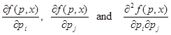
Gradients about the minimum
|
public double[][] getGrad()
|
|
Nelder and Mead Simplex Coefficients
|
public void setNMreflect(double reflectC)
|
|
public double getNMreflect()
|
|
public void setNMextend(double extendC)
|
|
public double getNMextend()
|
|
public void setNMcontract(double contractC)
|
|
public double getNMcontract()
|
|
See Common methods for list of methods associated with performing a non-linear regression, e.g. returning a statistical analysis of a non-linear regression, plotting the best fit curve.
|
|
Fitting data to special Functions
|
Scaling of the ordinate values
|
public void setYscaleFactor(double scaleFactor)
|
public void setYscaleOption(boolean test)
|
public boolean getYscaleOption()
|
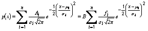
Fit to a Gaussian distribution
(parameter fixing option available)
or to Gaussian distributions
[normal distribution]
|
public void gaussian()
|
|
public void gaussian(double[] parameterValues, boolean[] fixedOptions)
|
|
public void gaussianPlot()
|
|
public void gaussianPlot(double[] parameterValues, boolean[] fixedOptions)
|
|
public void multipleGaussiansPlot(int nGaussians, double[] guessesOfMeans, double[] guessesOfStandardDeviations, double[] guessesOfFractionalContributions)
|
|
public static void fitOneOrSeveralDistributions(double[] array)
|
|
See also the ProbabiltyPlot class methods under Gaussian Probabilty Plot |
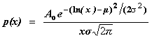
Fit to a Log-normal distribution
(two parameter statistic)
|
public void logNormal()
public void logNormalTwoPar()
|
public void logNormalPlot()
public void logNormalTwoParPlot()
|
|
public static void fitOneOrSeveralDistributions(double[] array)
|
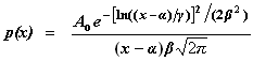
Fit to a Log-normal distribution
(three parameter statistic)
|
public void logNormalThreePar()
|
|
public void logNormalThreeParPlot()
|
|
public static void fitOneOrSeveralDistributions(double[] array)
|
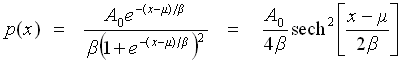
Fit to a Logistic distribution
|
public void logistic()
|
|
public void logisticPlot()
|
|
public static void fitOneOrSeveralDistributions(double[] array)
|
|
See also the ProbabiltyPlot class methods under Logistic Probabilty Plot |
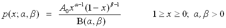
Fit to a Beta distribution
|
public void beta()
|
|
public void betaPlot()
|
|
public void betaMinMax()
|
|
public void betaMinMaxPlot()
|
|
public static void fitOneOrSeveralDistributions(double[] array)
|
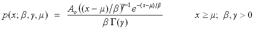
Fit to a Gamma distribution
|
public void gamma()
|
|
public void gammPlot()
|
|
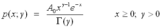
public void gammaStandard()
|
|
public void gammaStandardPlot()
|
|
public static void fitOneOrSeveralDistributions(double[] array)
|
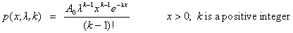
Fit to an Erlang distribution
|
public void erlang()
|
|
public void erlangPlot()
|
|
public static void fitOneOrSeveralDistributions(double[] array)
|
Fit to a Poisson distribution
|
public void poisson()
|
|
public void poissonPlot()
|
Fit to a Lorentzian distribution
|
public void lorentz()
|
|
public void lorentzPlot()
|
|
public static void fitOneOrSeveralDistributions(double[] array)
|
Fit to a Type 1 Extreme Value Distribution
(minimum order statistic)
Gumbel Distribution (minimum order statistic)
|
public void gumbelMin()
|
|
public void gumbelMinPlot()
|
|
public void gumbelMinOnePar()
|
|
public void gumbelMinOneParPlot()
|
|
public void gumbelMinStandard()
|
|
public void gumbelMinStandardPlot()
|
|
public static void fitOneOrSeveralDistributions(double[] array)
|
|
See also the ProbabiltyPlot class methods under Gumbel (minimum order statistic) Probabilty Plot |
Fit to a Type 1 Extreme Value Distribution
(maximum order statistic)
Gumbel Distribution (maximum order statistic)
|
public void gumbelMax()
|
|
public void gumbelMaxPlot()
|
|
public void gumbelMaxOnePar()
|
|
public void gumbelMaxOneParPlot()
|
|
public void gumbelMaxStandard()
|
|
public void gumbelMaxStandardPlot()
|
|
public static void fitOneOrSeveralDistributions(double[] array)
|
|
See also the ProbabiltyPlot class methods under Gumbel (maxiimum order statistic) Probabilty Plot |
Fit to a Type 2 Extreme Value Distribution
Fréchet distribution
|
public void frechet()
|
|
public void frechetPlot()
|
public void frechetTwoPar()
|
|
public void frechetTwoParPlot()
|
public void frechetStandard()
|
|
public void frechetStandardPlot()
|
|
public static void fitOneOrSeveralDistributions(double[] array)
|
|
See also the ProbabiltyPlot class methods under Fréchet Probabilty Plot |
Fit to a Type 3 Extreme Value Distribution
Weibull distribution
|
public void weibull()
|
|
public void weibullPlot()
|
public void weibullTwoPar()
|
|
public void weibullTwoParPlot()
|
public void weibullStandard()
|
|
public void weibullStandardPlot()
|
|
public static void fitOneOrSeveralDistributions(double[] array)
|
|
See also the ProbabiltyPlot class methods under Weibull Probabilty Plot |
Fit to a Type 3 Extreme Value Distribution (see also fitting simple exponentials)
Exponential Distribution
|
public void exponential()
|
|
public void exponentialPlot()
|
public void exponentialOnePar()
|
|
public void exponentialOneParPlot()
|
public void exponentialStandard()
|
|
public void exponentialStandardPlot()
|
|
public static void fitOneOrSeveralDistributions(double[] array)
|
|
See also the ProbabiltyPlot class methods under Exponential Probabilty Plot |
Fit to a Type 3 Extreme Value Distribution
Rayleigh Distribution |
public void rayleigh()
|
|
public void rayleighPlot()
|
|
public static void fitOneOrSeveralDistributions(double[] array)
|
|
See also the ProbabiltyPlot class methods under Rayleigh Probabilty Plot |
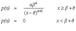
Pareto Distribution
|
public void paretoShifted()
|
|
public void paretoShiftedPlot()
|
|
public void paretoTwoPar()
|
|
public void paretoTwoParPlot()
|
|
public void paretoOnePar()
|
|
public void paretoOneParPlot()
|
|
public static void fitOneOrSeveralDistributions(double[] array)
|
|
See also the ProbabiltyPlot class methods under Pareto Probabilty Plot |
Fit to one or several of the above distributions
|
public static void fitOneOrSeveralDistributions(double[] array)
|
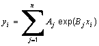
Fitting Simple Exponentials (See also fit to an Exponential Distribution)
yi = a.exp(b.xi)
yi = Σaj.exp(bj.xi)
yi = a.(1 - exp(b.xi))
|
public void exponentialSimple()
|
|
public void exponentialSimplePlot()
|
|
public void exponentialMultiple(int nExp)
|
|
public void exponential|MultiplePlot(int nExp)
|
|
public void exponentialMultiple(int nExp, double[] initialEstimates)
|
|
public void exponential|MultiplePlot(int nExp, double[] initialEstimates)
|
|
public void oneMinusExponential()
|
|
public void oneMinusExponentialPlot()
|
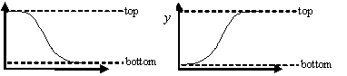
Fit to a Sigmoid Function
Sigmoidal Threshold Function
|
public void sigmoidThreshold()
|
|
public void sigmoidThesholdPlot()
|
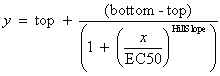
Fit to a Sigmoid Function
Hill/Sips Sigmoid
|
public void sigmoidHillSips()
|
|
public void sigmoidHillSipsPlot()
|
Fit to a Sigmoid Function
Five parameter logistic curve
[5PL]
|
public void fiveParameterLogistic()
|
|
public void fiveParameterLogisticPlot()
|
|
public void fiveParameterLogistic(double bottom, double top)
|
|
public void fiveParameterLogisticPlot(double bottom, double top)
|
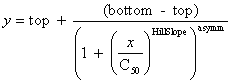
Fit to a Sigmoid Function
Four parameter logistic curve
[4PL, EC50 dose response curve]
|
public void fourParameterLogistic()
|
|
public void ec50()
|
|
public void fourParameterLogisticConstrained()
|
|
public void ec50constrained()
|
|
public void fourParameterLogisticPlot()
|
|
public void ec50Plot()
|
|
public void fourParameterLogisticConstrainedPlot()
|
|
public void ec50constrainedPlot()
|
|
public void fourParameterLogistic(double bottom, double top)
|
|
public void ec50(double bottom, double top)
|
|
public void fourParameterLogisticPlot(double bottom, double top)
|
|
public void ec50Plot(double bottom, double top)
|
Fit to a Rectangular Hyperbola
|
public void rectangularHyperbola()
|
|
public void rectangularHyperbolaPlot()
|
public void shiftedRectangularHyperbola()
|
|
public void shiftedRectangularHyperbolaPlot()
|
Fit to a Scaled Heaviside
Step Function
|
public void stepFunction()
|
|
public void stepFunctionPlot()
|
Common instance methods
(see below for common
static methods)
|
Input data option
|
public void setErrorsAsScaled();
|
|
public void setErrorsAsSD();
|
|
public void setTrueFreq(boolean trueOrfalse)
|
|
public boolean getTrueFreq()
|
Add a title to graphs
and output files
|
public void setTitle(String title)
|
|
Print the regression results
|
public void print( String filename, int prec)
|
|
public void print( String filename)
|
|
public void print(int prec)
|
|
public void print()
|
Suppress the printing of
the regression results
|
public void suppressPrint()
|
Plot the regression results
x against y
|
public int plotXY( String graphName)
|
|
public int plotXY()
|
|
public int plotXY(RegressionFunction rf, String graphName)
|
|
public int plotXY(RegressionFunction2 rf, String graphName)
|
|
public int plotXY(RegressionFunction3 rf, String graphName)
|
|
public int plotXY(RegressionFunction rf) |
|
public int plotXY(RegressionFunction2 rf) |
|
public int plotXY(RegressionFunction3 rf) |
Plot the regression results
y(exp) against y(calc)
|
public int plotYY(String filename)
|
|
public int plotYY()
|
Suppress the plot of the regression
results y(exp) against y(calc)
|
public void suppressYYplot()
|
|
Add axis legends to the x - y plot
|
public void setXlegend(String xLegend)
|
|
public void setYlegend(String yLegend)
|
|
Return the best estimates
|
public double[] getBestEstimates()
|
|
Return the errors of the best estimates
|
public double[] getBestEstimatesErrors()
|
|
Return the coefficients of variation
|
public double[] getCoeffVar()
|
|
Return the t-values of the best estimates
|
public double[] getTvalues()
|
|
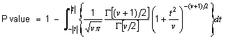
Return the P-values of the best estimates
|
public double[] getPvalues()
|
|
Return the calculated y values
|
public double[] getYcalc()
|
|
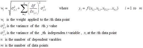
Return the weights
|
public double[] getWeights()
|
|
Return the unweighted residuals
|
public double[] getResiduals()
|
|
Return the weighted residuals
|
public double[] getWeightedResiduals()
|
|
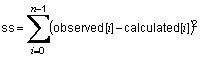
Return the unweighted sum of residual squares
|
public double getSumOfSquares()
public double getSumOfUnweightedResidualSquares()
|
|
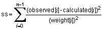
Return the weighted sum of residual squares
|
public double getChiSquare()
public double getSumOfWeightedResidualSquares()
|
|
Return the reduced chi square
|
public double getReducedChiSquare()
|
|
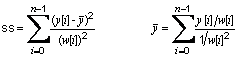
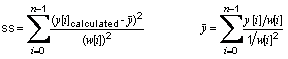
Return the total sum of weighted squares
|
public double getTotalSumOfWeightedSquares()
|
|
Return the regression sum of weighted squares
|
public double getRegressionSumOfWeightedSquares()
|
|
Return the linear correlation coefficient
|
public double getXYcorrCoeff()
public double getYYcorrCoeff()
|
|
Return the coefficient of determination
|
public double getCoefficientOfDetermination()
|
|
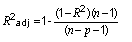
Return the adjusted coefficient of determination
|
public double getAdustedCoefficientOfDetermination()
|
|
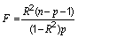
Return the coefficient of determination F-ratio
|
public double getCoeffDeterminationFratio()
|
|
Return the coefficient of determination F-ratio probability
|
public double getCoeffDeterminationFratioProb()
|
|
Return the degrees of freedom
|
public int getDegFree()
|
|
Covariance Matrix
|
public double[ ][ ] getCovMatrix()
|
|
Parameter correlation coefficients
|
public doublet[ ][ ] getCorrCoeffMatrix()
|
|
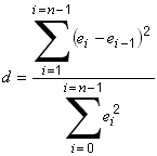
Return the Durbin-Watson d Statistic
|
public double getDurbinWatsonD()
|
|
Check normality of residuals
|
public void checkResidualNormality()
|
|
public void checkWeightedResidualNormality()
|
|
Common static methods
|
Test of additional terms
(Extra sum of squares)
|
public static ArrayList<Object> testOfAdditionalTerms(double chiSquare1, int nParameters1, double chiSquare2, int nParameters2, int nPoints, double significanceLevel)
|
|
public static ArrayList<Object> testOfAdditionalTerms(double chiSquare1, int nParameters1, double chiSquare2, int nParameters2, int nPoints)
|
|
public static ArrayList<Object> testOfAdditionalTerms_ArrayList(double chiSquare1, int nParameters1, double chiSquare2, int nParameters2, int nPoints, double significanceLevel)
|
|
public static ArrayList<Object> testOfAdditionalTerms_ArrayList(double chiSquare1, int nParameters1, double chiSquare2, int nParameters2, int nPoints)
|
|
public static double testOfAdditionalTermsFratio(double chiSquare1, int nParameters1, double chiSquare2, int nParameters2, int nPoints)
|
|
public static double testOfAdditionalTermsFprobability(double chiSquare1, int nParameters1, double chiSquare2, int nParameters2, int nPoints)
|
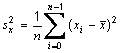
Resetting the denominator in statistical formulae
|
public static void setDenominatorToN()
|
public static void setDenominatorToNminusOne()
|
Reset Stat class continued fraction evaluation parameters
This evaluation is called by the Regression statistical analysis
|
public static void resetCFmaxIter(int maxit)
|
public static int getCFmaxIter()
|
public static void resetCFtolerance(double tolerance)
|
public static double getCFtolerance()
|